Artificial Intelligence, Competition, and Welfare

PDF Page 1

NBER WORKING PAPER SERIES

ARTIFICIAL INTELLIGENCE, COMPETITION, AND WELFARE

Susan Athey Fiona Scott Morton

Working Paper 34444 http://www.nber.org/papers/w34444

NATIONAL BUREAU OF ECONOMIC RESEARCH

1050 Massachusetts Avenue Cambridge, MA 02138

November 2025

Susan Athey previously served as chief economist of the antitrust division of the U.S. Department of Justice. She has worked on various consulting cases for a variety of clients through Keystone Strategy. She is the founding faculty director of the Golub Capital Social Impact Lab. Fiona Scott Morton engages in consulting on issues related to antitrust and mergers. In the last three years she has consulted for Microsoft corporation and NVIDIA on competition topics unrelated to AI. The research reported in this paper is independent academic work, is unrelated to any consulting matters, and has not been funded by any entity apart from Yale University. The views expressed herein are those of the authors and do not necessarily reflect the views of the National Bureau of Economic Research.

NBER working papers are circulated for discussion and comment purposes. They have not been peer-reviewed or been subject to the review by the NBER Board of Directors that accompanies official NBER publications.

© 2025 by Susan Athey and Fiona Scott Morton. All rights reserved. Short sections of text, not to exceed two paragraphs, may be quoted without explicit permission provided that full credit, including © notice, is given to the source.

PDF Page 2

Artificial Intelligence, Competition, and Welfare Susan Athey and Fiona Scott Morton NBER Working Paper No. 34444 November 2025 JEL No. L10, L12, L4, L40, L5

ABSTRACT

We study how market power in artificial intelligence (AI) shapes wages and welfare in openeconomy general equilibrium by treating AI as a priced, imported factor. Across three models, we separate technical efficiency from the impact of upstream price setting. In a two-traded-goods benchmark, the incidence of AI price changes depends on how sectoral skill intensity changes with AI prices; non-monotone intensity can generate “double harm” for unskilled workers (lower real wage after a large decrease in the price of AI, and real wage decreases further when the AI price rises as a result of market power). With one non-traded sector, we observe that the classic “Dutch disease” effect here would arise when one sector gets more productive and draws labor away from other sectors, creating scarcity and raising prices; but this is not what we expect from the introduction of labor-substituting AI. In contrast, our last model considers two non-traded sectors and CES/free entry, and the opportunity for discrete adoption of technology that replaces unskilled labor from the AI-using sector. When AI reduces unit costs and increases variety, it will not pull U from non-tradables, instead it will displace workers from the AI-using sector and lower wage due to diminishing returns in alternative sectors. Strategic upstream pricing of AI then harms welfare through unit-cost (usage fees) and variety (access fees) channels, with income leakage abroad. We derive an adoption frontier tying feasible usage prices to displaced workers’ outside options and show a monopolist typically prices on this boundary; capping one instrument shifts rents to the other. Broad gains for the adopting country relies on pressure (or regulation) on both usage and access fees and as well as policy that supports productive absorption of displaced labor. The framework clarifies when AI can lower real wages and aggregate welfare despite efficiency gains.

Susan Athey Stanford University Graduate School of Business Department of Economics and NBER athey@stanford.edu

Fiona Scott Morton Yale University Yale School of Management and NBER fiona.scottmorton@yale.edu

PDF Page 3

Introduction

Economists have observed that artificial intelligence (AI) may have a variety of downstream benefits for the economy: it may improve productivity, enable innovation and the entry of new firms, and it may be used to reduce switching costs, eroding the market power of existing firms. While recognizing the potential benefits of AI, regulators also grapple with its risks. In addition to concerns about war and democracy, there are economic risks such as worker displacement and industry reorganization that affect distribution within and across countries. In this paper, we focus on the relationship between these risks and what we view as a critical factor affecting the balance of benefits and risks: market power in AI. Competition authorities worldwide have recognized that AI may create new bottlenecks, leading to higher prices, reduced innovation, and lower benefits for consumers. The UK’s Competition and Markets Authority, the US FTC, and other agencies have issued reports and are monitoring commercial relationships within the AI stack.1

Scrutiny is warranted because different layers of the AI stack—from chips to foundation models to applications and distribution channels—exhibit concentration. Examples include NVIDIA’s dominance in advanced chips, concentration among foundation model providers (OpenAI, Gemini, Claude), and the dependence of downstream applications (e.g. search engines, language tutors, writing assistants, customer service platforms, document search tools) on a few foundation models. Access to data that is crucial for AI performance may be gated by incumbents in both the consumer and enterprise software markets. Distribution channels, such as mobile operating systems, productivity software, and online platforms, are especially concerning given their entrenched power. When these channels are controlled by firms that also supply AI or search, entrants face foreclosure risk, and even highly efficient AI applications can struggle to gain distribution (as was publicly argued by Perplexity in 2025 in the context of the Google search remedies discussion, e.g. Vasant [2025]). Competition enforcers are particularly wary of underenforcement in AI, recalling slow responses to earlier digital platform monopolization (Google in search and ads, Meta in social networking, Amazon in e-commerce, Apple and Google in mobile ecosystems). In those cases, delayed enforcement allowed monopolies to entrench themselves. In the case of AI, by contrast, agencies are proactively investigating potential harms while the market remains in flux. This approach may be especially important because AI is a general-purpose technology, meaning any monopoly harm will extend well beyond a single sector. Having said that, the enforcement tools available to antitrust authorities are limited, and enforcement may be misdirected or ineffective. The general equilibrium framework introduced in this

1[Competition and Markets Authority, 2023, 2024, Portuguese Competition Authority, 2023]

PDF Page 4

paper formalizes the economy-wide consequences of unchecked market power.

In this paper, we argue that the extent to which the artificial intelligence (AI) industry provides services to traditional industries at competitive, low prices has critical implications for the impact of AI on income distribution and welfare. To do so, we consider extensions and variants of standard general equilibrium and trade models, highlighting how different assumptions about the nature of technology, the productive alternative uses of labor, and the aggregate market power in the artificial intelligence stack leads to different conclusions about whether real wages for different categories of workers rise or fall. Unlike much of the literature that focuses primarily on distribution, we consider assumptions that are rich enough such that productivity improvements from AI do not necessarily result in improvements in economy-wide welfare, let alone welfare for specific groups.

By focusing on a limited set of extensions to existing models, we are able to highlight novel forces that arise with different assumptions in familiar modeling frameworks, but our view is that future research may productively expand the set of models to better match possible impacts of the introduction of AI. For example, AI may make it difficult for some groups of workers to transition from shrinking sectors to growing ones, for countries to increase exports at fixed prices, and for citizens to maintain influence over government policies. Future research might also provide a deep analysis of incentives for innovation as well as industrial policies and policies around the procurement and provision of government services that strategically position countries to benefit as much as possible, and mitigate harm, from AI. But in this paper our goal is primarily to set up some of the key forces and highlight the tradeoffs that we believe advance a critical research agenda.

Specifically, this paper develops formal models to study how the arrival and pricing of artificial intelligence (AI) services affect wages, output, and welfare. To do so, we observe that the arrival of a new technology can be modeled similarly to the availability of a new input factor available through trade. Thus, we analyze the impact of AI using models of a small economy, considering cases of open and closed economies. However, we include a competition element in the model by treating AI as an intermediate input X supplied either by a foreign monopolist, supplied competitively, or somewhere in between. The price pX of AI is therefore not a world price taken as given, but a strategic variable chosen by the upstream supplier, where the supplier may set the price to maximize revenue, but may also be constrained by policy. The goal is to understand how the introduction of AI (moving pX from ∞to a finite level) and subsequent changes in its price redistribute income across factors, shift output, and affect aggregate welfare. We are particularly interested in what happens to real wages for workers, and whether high prices for AI lead to reductions in the real wage despite efficiency benefits in production. In extensions, we highlight the particularly challenging but realistic

PDF Page 5

scenario where AI providers can use nonlinear pricing schemes, influencing entry, innovation and industry structure in downstream industries.

In our models the supplier of AI may be able to extract the surplus created by AI technology, while, at the same time, the exercise of market power inflicts additional loss on the workers displaced by the AI. This contrasts with a standard model where, if a technology is introduced that disproportionately displaces a group of workers, raising prices for the input helps that group by diminishing the substitution.

We also highlight the key question of whether other sectors, either non-traded sectors or export sectors, can productively absorb displaced workers, an assumption that may be questionable in the face of a major technological shift. This focus underscores the critical role played by government policies that change how productive workers are in sectors less affected by AI. For example, the government may increase spending on services that benefit society and then help displaced workers transition into those industries. In many countries education, health care, policing, or child and elder care are consumed at levels too low for citizens to achieve their potential in production. Government policy can affect reskilling in these areas, and AI can be used to help workers become more productive in new roles.

The popular interest in AI has stimulated a macroeconomic literature modeling the possible faster growth in several ways. For example, Aghion et al. [2019] embed AI into standard growth frameworks to explore implications for the labor–capital ratio and the share of expenditure on automated tasks. Outcomes depend on parameters such as substitution elasticities between automated and non-automated goods, the speed of cost reductions for automated goods, and the proportion of tasks that can be automated. Nordhaus [2021] provides a clear treatment of the channels through which AI can increase economic growth. He presents a model in which AI induces capital deepening, which in turn accelerates growth. Nordhaus emphasizes that returns accrue primarily to capital: “Capital eventually gets virtually all the cake, but the crumbs left for labor—which are really small pieces of the increasingly huge mountains of cake—are still growing at a phenomenal rate” (p. 14).

Studies of task–based and automation frameworks (e.g., Autor et al., 2003, Acemoglu and Restrepo, 2018, 2020, Autor and Salomons, 2018, Autor and Thompson, 2025) study how technology displaces or complements labor when technology costs and output prices are taken as parametric. Growth papers embed AI as a driver of factor usage and total factor productivity (e.g., Aghion et al., 2019, Nordhaus, 2021); open-economy work on directed technical change treats final goods as traded and incidence of impacts as disciplined by terms-of-trade movements (e.g., Korinek and Stiglitz, 2018, 2021). Our Model 1 nests that benchmark. The new forces we emphasize—AI as a priced, imported factor with upstream market power and endogenous adoption—require letting pX be strategic and allowing non-

PDF Page 6

tradables to affect the CPI, so that aggregate income gains and real-wage losses can coexist.

A second strand of research connects to Dutch-disease and non-tradables [Corden and Neary, 1982, Corden, 1984]: here the “boom” in B is not a free endowment but requires paying pX, so income can leak abroad.

Korinek and Stiglitz [2018, 2021] propose a series of models that focus on distributional consequences and policy responses from exogenous technological shocks or changes in the returns to the resources of small countries. A complementary line of work, going back to Stiglitz [1976] and further developed in Delli Gatti et al. [2012], Gatti et al. [2012], studies dual-economy settings in which a constant-returns agricultural sector coexists with an urban sector featuring wage rigidity (e.g., due to efficiency-wage considerations). In their baseline environment, an agricultural productivity improvement is unambiguously welfare-reducing: higher rural productivity contracts urban employment when nominal wages cannot adjust, and with flexible wages an induced wage decline can further depress demand and raise unemployment. Although entrepreneurs may gain from lower wages, inequality-averse social welfare functions imply aggregate welfare losses. Our models connect to these results but identify distinct channels that do not rely on nominal rigidities.

Overall, these literatures do not consider jointly the overall and distributional impacts of the technology together with how the technology is priced. Additionally, in a typical growth model both the technology and the workers are located in the same economy.

Our contribution is to bring a trade/general equilibrium approach to analyzing AI, treating AI as a priced, imported factor whose upstream market power (and tariff–like instruments) is central. This allows us to separate (i) pure technological efficiency from (ii) the impact of the price path of AI services and the corresponding changes in factor markets and input markets, and to ask how welfare depends jointly on whether AI prices fall with productivity and on whether displaced workers are sufficiently productive in sectors less affected by AI. We show that conclusions about wages and aggregate welfare turn on a small set of modeling choices—whether goods are traded versus non-traded (and in turn, whether there are diminishing marginal utility in the output markets), whether automation reduces demand for some or all groups of labor to (near) zero so that output expansions in newly productive industries do not lead to increases in labor demand, and whether the upstream supplier can use nonlinear pricing—that are especially salient for AI. A recurring theme is that some familiar GE mechanisms are not first-order when automation in B removes unskilled labor (so uB →0). In that case, “Dutch-disease” style labor-pull out of the non-traded sector is mechanically weaker, and the key margins instead become the price index in B (via mB and variety) and income leakage to a foreign AI provider. Our third model is designed to surface precisely these forces.

PDF Page 7

We proceed by developing a sequence of three models, highlighting mechanisms in each model and noting where they do or do not match what we might expect in the case of AI. We then discuss policy conclusions and open research questions, taking the perspective that the simple models we propose are only a start at answering key policy questions.

Throughout, the price of AI, denoted pX, is a strategic object, and firms and market outcomes respond to it. Even holding the technology set fixed, changing pX reallocates income between factors and shifts national income. This “price versus technology” distinction underpins our richer models when output and variety are endogenous. However, we can think of large changes in price as very similar to a change in technology, since at different prices, different values of the factor will be chosen, and the cost-minimizing choice of factors and equilibrium wages can shift qualitatively. We consider both continuous and discrete production functions, where a large fall in the price of an AI input may fundamentally change which factor of production (e.g. skilled or unskilled labor) is dominant, and where labor demand may be insensitive to input prices for technologies that fully automate. We also pay special attention to the choices firms make about adopting AI in the face of a strategic monopolist setting prices for the AI input to extract surplus.

Model 1: AI as a new factor in a small economy with

two traded goods.

We begin with the standard two–good Heckscher–Ohlin model. Sector A produces using skilled and unskilled labor (LS, LU) alone; sector B combines (LS, LU) with AI, purchased at price pX from the foreign supplier. We write the quantity of labor type i ∈{S, U} in sector j ∈{A, B} as ij. Both goods A and B are traded at exogenous world prices (¯pA, ¯pB). When pX = ∞, AI is unavailable and the economy collapses to the benchmark two–sector HO model. When pX is finite, sector B’s costs cB depend on (wS, wU, pX), where (wS, wU) are the equilibrium wages of skilled and unskilled labor. Throughout, we measure the AI input price pX in units of the traded good B (normalizing ¯pB = 1), so payments to the foreign supplier are valued at world prices.

In this all–traded setting, zero–profit conditions determine (wS, wU) as a function of pX. The Stolper–Samuelson mapping implies that one wage rises while the other falls when pX changes; which factor gains depends on the relative intensity of A and B. Formally, for each sector j ∈{A, B}, let θj

i = wiaj

i/cj denote the cost share of factor i ∈{S, U}, and let Rj = θj

S/θj

U denote the sectoral intensity ratio. B is skill–intensive relative to A if RB > RA, and unskilled–intensive if RB < RA.

PDF Page 8

We assume that for sufficiently high pX, sector B’s skill intensity RB(pX) := θB

S /θB

U is decreasing in pX (equivalently, increasing as AI gets cheaper). A stronger condition that we refer to in some results is strong substitutability (SS) of X for unskilled labor in B, under which the Hicksian unit demand aB

U falls as pX falls and, for low enough pX, aB

U →0; SS implies R′

B(pX) < 0 for all pX and ensures there is at most one crossing of RB with RA as we vary pX.

General-equilibrium mapping and reallocation. Totally differentiating zero-profit in A and B at fixed (¯pA, ¯pB) yields

θA

S dwS + θA

U dwU = 0, θB

S dwS + θB

U dwU + θB

X dpX = 0.

Eliminating dwU,

�

θB

S −θB

θA

S θA

�

dwS = −θB

X dpX,

=⇒ sign

� dwU

dpX

�

= sign(RB −RA), sign

� dwS

dpX

�

= −sign(RB −RA).

(GE)

This highlights that a change in pX affects RB through both substitution across sectors as well as across factors. If B is unskilled-intensive (RB < RA) and pX increases, then wS rises and wU falls; activity tilts from B toward A (which is relatively more skill-intensive). Applying the envelope theorem to national income (NI), we have dY

dpX = −MX ≤0: increasing pX decreases income.

How do the introduction of AI and the exercise of market power affect workers? Case A: RB decreasing in pX everywhere and B skill-intensive everywhere (RB > RA). From (GE), dwU

dpX > 0 at all finite pX: raising pX helps unskilled workers. Thus the introduction of AI (moving from autarky pX = ∞to any finite pX) is bad for unskilled workers, while starting from a low pX, an increase in pX benefits them locally. (Skilled wages move in the opposite direction: dwS dpX < 0.) Case B: RB decreasing in pX and crossing RA once as pX rises (from skill- to unskilledintensive). Now consider the case where in autarky, Sector B is unskilled-intensive, but as pX drops, X substitutes for unskilled workers and eventually at low pX the sector is skilled-intensive. Then, there exists p∗

X with RB > RA for pX < p∗

X and RB < RA for pX > p∗

• For low pX (where B is skill-intensive), dwU dpX > 0: At low prices, the introduction/expansion of AI can be bad for unskilled workers, if the area of skill-intensity is large enough; but

PDF Page 9

anywhere this area is large enough occurs at prices where RB > RA and so increasing pX helps them.

• For high pX (where B is unskilled-intensive), dwU dpX < 0: unskilled workers are helped by the introduction of AI, but locally hurt by an increase in pX.

In summary, if as pX ↓0 the unit demand aB

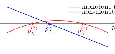
U →0—Sector B becomes more skill intensive as AI gets cheaper. In this monotone case there can be at most a single intensity reversal at some p∗

X where RB(pX) = RA. Around such a single reversal, the local effect of a small change in pX and the global level effect relative to autarky need not align: near p∗

X the level effect for unskilled workers is positive on both sides (opening to moderately cheap AI benefits them overall), while the local derivative flips sign at p∗

X (so a price increase in AI can either help or hurt them depending on the side). This is the familiar trade intuition that the losers from ongoing technology adoption in the skill-intensive region may be locally helped by a higher pX (e.g., a tariff or a markup reversal). However, if unskilled workers are hurt by the introduction of AI, the prices must be low enough that Sector B is skill-intensive, so that higher pX helps them.

dwU

dpX

0 p(2)

X p(1)

X p∗

monotone (single crossing) non-monotone (double crossing)

Figure 1: Local incidence of AI input prices on the unskilled wage: dwU

dpX vs. pX. Above the zero line, unskilled wages rise with pX; below, they fall. A monotone path yields a single crossing (blue), while a non-monotone path yields two (red).

Double vs. single reversals. RB(pX) need not be monotone. For example, sector B may be able to choose among multiple techniques with different optimal unit skill requirements (ak

S, ak

U, ak

X). A natural pattern is: in autarky B is relatively unskilled–intensive; as pX falls it becomes skill–intensive (AI substitutes for unskilled tasks); and at very low pX AI substitutes strongly for both types of labor so B again looks unskilled–intensive:

RB < RA (pX very high), RB > RA (pX intermediate), RB < RA (pX very low).

With two crossings of RA, the introduction of AI supplied by a firm with market power

PDF Page 10

can deliver a “double-harm” to unskilled workers: for sufficiently low pX, the unskilled wage can lie below its autarky value and be locally decreasing in pX. The local decrease arises because at those very low prices B is again unskilled–intensive relative to A, so a higher pX reduces B’s output and differentially reduces demand for unskilled labor.

This highlights that the shape of RB(pX) is critical for who is helped and hurt by input price changes. At the aggregate level, the country gains from cheaper AI (by the envelope result dY/dpX = −MX ≤0), and one group’s loss is the other’s gain via the Stolper–Samuelson mapping.

Model 2: One traded, one non-traded good.

We then extend Model 1 by making A non-traded and closing the economy with Cobb– Douglas preferences over (A, B): U = C1−α

A Cα

B, where Cj is consumption of sector j. As A is non-traded, we must have CA equal to the output of A, QA.

This extension provides several additional mechanisms to analyze. First, this change endogenizes the non-traded price pA through market clearing and introduces a novel income– demand–price channel on top of the Stolper–Samuelson logic, the classic “Dutch-disease” mechanism: as B scales, resources shift out of A, so QA decreases and pA = (1−α)Y

QA , increases. This raises the CPI and can lower both groups’ real wages.

To see this in more detail, first recall that the fact that B is exported and the country is small induces the country to shift into exports of B when that industry gets more productive. Because household utility is Cobb–Douglas, aggregate expenditure equals domestic absorption, that is, domestic production net of AI imports:

Y = pAQA + ¯pBQB −pXMX,

where Y is national income (the wage bill plus rebates), QB is output of B, and MX are AI imports. The consumption price index is

P = p 1−α

A ¯p α

B, pA = (1 −α)Y

so both factors’ real wages share a common cost-of-living term because both types of workers purchase more expensive A goods as a share 1 −α of expenditure. If pA rises sharply when resources reallocate to increase production of B and decrease production in A, both real wages can fall simultaneously—an outcome that is impossible when all goods are traded. We emphasize that this mechanism depends on B actually pulling labor from A—an as-

PDF Page 11

sumption that may be inappropriate when AI removes unskilled workers from B’s marginal cost (motivating modifications to the setup in Model 3).

Second, allowing a non-traded good (so that the CPI is endogenous) creates a channel that can generate a double-harm for unskilled labor. In the two-traded-goods benchmark, if RB(pX) is monotone, then whenever a fall in pX (the “cheap-AI” move) leaves unskilled workers worse off in levels at the new equilibrium, a marginal increase in pX at that point must raise their (nominal and real) wage—the local and global effects necessarily have opposite signs; only with a non-monotone RB path can both effects be adverse.

With a non-traded closure, the CPI adds a wedge: P = p1−α

A ¯pα

B (with ¯pB tied to world prices), so the local real-wage response is

d ln(wU/P) = d ln wU −(1 −α) d ln pA = d ln wU −(1 −α) (d ln Y −d ln QA).

Even if the nominal Stolper–Samuelson effect points one way (e.g., B is unskilled-intensive so d ln wU/d ln pX < 0), a sufficiently strong co-movement of the non-traded price with pX can overturn the sign of the real response:

d ln(wU/P)

d ln pX

< 0 ⇔ (1 −α) d ln pA

d ln pX

> d ln wU

d ln pX

Hence it is possible that (i) unskilled workers are worse off in levels at the low-pX (“cheapAI”) equilibrium relative to a high-pX benchmark, and (ii) the local derivative of their real wage with respect to pX at that point is negative—i.e., a marginal increase in pX would make them even worse off. In the Appendix we give sufficient conditions—in terms of (RA, RB(pX)) and the non-traded expenditure share 1−α—under which this alignment of global and local losses occurs.

Third, price increases by the AI provider (pX ↑) are now partially cushioned or amplified through movements in pA, depending on which sector is relatively factor-intensive. When a fall in pX expands B and contracts A, the non-traded price rises by the closure pA = (1 −α)Y/QA: higher income and lower QA both bid up pA. We can formally analyze the welfare ratio between an AI and no-AI regime as follows. By the envelope theorem,

dY dpX = −MX, and further:

U ∗AI

U ∗0 =

�Y ∗AI

Y ∗0

�α �Q∗AI

A Q∗0

�1−α

In applications, the two sufficient statistics, MX/Y and 1 QA

dQA

dpX , provide a diagnostic: if the latter is small because B’s expansion does not reduce QA, the income gain from cheaper AI

PDF Page 12

dominates; if it is large and positive, CPI pressures can overturn income gains.

These mechanisms connect our model to the classic Dutch disease and real-exchange-rate literatures [e.g. Corden and Neary, 1982, Corden, 1984, Burstein et al., 2003, Corsetti et al., 2008].2, which emphasize how a resource boom or terms-of-trade improvement raises national income but simultaneously appreciates non-tradables, reallocating factors to e.g. exports and raising the cost of living. The novelty in our analysis is to embed these price-index channels in a small-open-economy model that captures the introduction of a new technology, AI, sold by a foreign supplier with market power. Here the comparative static is with respect to AI pricing, not a resource windfall. This shift allows us to characterize welfare and distributional incidence in transparent sufficient statistics: import exposure MX/Y and non-traded scarcity elasticities dQA/dpX.

Two features of Model 2 can overstate CPI pressures in Sector A as a result of AI. First, if automation in B makes uB ≈0, scaling B need not pull unskilled labor out of A; the mechanical shift of resources out of Sector A may not occur, and pA may rise less (or not at all). Second, treating the good from B as traded at an exogenous world price abstracts from the possibility that AI adoption is global, limiting a small country’s ability to expand B at fixed ¯pB. Next, we introduce Model 3 that addresses both issues by (i) making B non-traded with CES/entry (so the price index moves through unit-cost and variety) and (ii) modeling discrete adoption that eliminates unskilled workers from B (uB →0).

Model 3: Discrete Technology Adoption with Two Non-

traded Sectors

As in Model 2, in Model 3 households have Cobb–Douglas preferences over two goods, so both types of workers face a common CPI. Here, however, two new features are introduced. First, both sectors are non–traded, so there is no world-price anchor: both PA and PB are determined domestically. Second, sector B consists of many differentiated varieties under CES demand (elasticity σ > 1) with constant markup µ = σ/(σ −1) > 1 and free entry subject to a per-firm domestic license fee F (rebated lump-sum to households) and a fixed access charge, ϕ, that is collected by the foreign monopolist.

Primitives and price indices. Households spend a constant share α ∈(0, 1) on B and 1 −α on A: U = C 1−α

A C α

B , EB = αY, EA = (1 −α)Y. (1)

2See also ?Chari et al. [2002], De Gregorio and Wolf [1994].

PDF Page 13

Within B, symmetry across the N active firms implies

QB =

� N X

i=1

σ−1

σ i

� σ

σ−1, PB =

� N X

i=1

p1−σ

� 1 1−σ = N 1 1−σ pB, (2)

and the CPI is

P = p 1−α

A p α

B. (3)

Without loss of generality, we normalize pA = 1 so that all prices are relative to the price index in Sector A; although at times we discuss the price effects in Sector A, these should be interpreted as relative prices.

Pricing and free entry in B. Let mB be the unit marginal cost and pB = µ mB the symmetric price. With per-firm outlays F + ϕ and free entry,

(pB −mB)q = (F + ϕ) ⇒ pB q = µ µ−1(F + ϕ). (4)

Because the expenditure in Sector B is EB = αY = NpBq, the number of active firms is

N = µ−1

µ α | {z }

Y F + ϕ, PB = µ mB

�

κ Y F + ϕ

� 1 1−σ . (5)

Thus, holding Y and (F + ϕ) fixed, changes in mB move pB but do not move N directly. In general equilibrium, however, pX and ϕ move Y and hence N through free entry. This yields a clear welfare decomposition: unit-cost (mB) and variety (N) effects are distinct levers, both sensitive to upstream market power.

It is natural to study AI adoption in a model with fixed costs because digital technologies and AI services often require substantial up-front investment (training, deployment, access) but then exhibit low marginal cost of use. A CES/free-entry structure captures this well: the number of firms N depends on income and fixed costs, not directly on marginal cost. This makes it possible to analyze how AI pricing reshapes industry structure (the equilibrium number of firms, variety, and the quality-adjusted price index). Moreover, because AI is a general-purpose technology that enables a wide range of applications, entry and variety are themselves first-order welfare channels. A CES environment highlights how monopolist pricing can distort not only wages and aggregate income but also the diversity of products consumers access. This goes beyond the simpler competitive frameworks and justifies the more complex setup.

PDF Page 14

AI technology and marginal cost in B. A foreign upstream supplier charges a per-firm access fee ϕ and a per-unit usage price pX (we start by setting ϕ = 0 to facilitate comparisons to Model 2, and then generalize the model). Adoption in B is discrete and takes one of two forms:

Partial automation: mB = sBwS + pX, Full automation: mB = pX. (6)

In both cases, adoption implies uB = 0, so displaced unskilled labor reallocates to A. In contrast to Model 2, because uB = 0, a marginal expansion of B need not pull U from A; instead, U is already in A and faces diminishing returns there. The CPI channel now runs primarily through pB (via mB and N), not through pA (via QA).

Sector A and factor markets. Sector A is produced competitively with both skilled and unskilled labor. With fixed endowments LS, LU,

S + LB

S = LS, LA

U + LB

U = LU, LB

U = 0 under adoption. (7)

With diminishing returns in A, the crowding of unskilled labor into A lowers wU, while wS reflects the allocation of LS across sectors and—under partial automation—the demand for LS in B.

Income and external payments. Domestic income includes wages and the rebated F (as in Model 2) but excludes foreign AI payments:

Y = wSLS + wULU + FN, Foreign outflow = ϕN + pXQB. (8)

In contrast to the case of the fixed cost F, if the foreign AI supplier charges a per–firm access fee ϕ (as we consider below), those payments do not recycle domestically. Unlike F, ϕ reduces both entry and domestic absorption, since the transfers are lost to the foreign monopolist.

Exogenous AI Prices

Adoption frontier defined. AI is adopted only if it beats the baseline when rivals adopt. As we discuss in more detail below, this yields a downward-sloping frontier of the set of incentive-compatible (ϕ, pX) pairs, where the frontier can be written as pX ≤pX,max(ϕ). Importantly, adoption constraints are more challenging when other firms adopt, since adoption frees up labor and pushes down wages. In this section, we first consider comparative statics

PDF Page 15

on usage and access fees within the frontier, and then return to consider the frontier in more detail when we consider the problem faced by a monopolist AI provider.

Equilibrium. Let Z−(α, σ, F, sB; LS, LU) denote the vector of exogenous primitives (preferences, technologies, and endowments) for Model 3. Given (Z, ϕ, pX), a (competitive) equilibrium consists of prices, quantities, and allocations

�

pA, PB, pB, mB, N, q, QB; wS, wU; LA

S, LB

S , LA

U, LB

U; Y

�∗r

where the superscript ∗r denotes equilibrium values in Model 3 for regime r ∈{AI, 0} (r = 0 being no AI), that jointly satisfy equations (1)-(8). When analyzing the monopolist’s problem, the feasible (ϕ, pX) must also satisfy the adoption frontier pX ≤pX,max(ϕ). For any equilibrium variable X in the list above, we use the superscript notation X∗r(Z, ϕ, pX) to denote its equilibrium value as a function of (Z, ϕ, pX).

Welfare Ratio In the Appendix, we show that substituting in equilibrium conditions and comparing the AI equilibrium to the no–AI baseline yields

W ∗AI

W ∗0 =

� m∗0

B m∗AI

�α

| {z } unit cost / B-side price index

� F F + ϕ

� α

σ−1

| {z } variety / entry

�Y ∗AI

Y ∗0

�α+ α σ−1

| {z } aggregate income

(9)

That is, the welfare ratio can be decomposed into the product of three ratios. The first is proportional to the ratio of marginal costs across regimes, which affects the welfare ratio through the price index; the second is the ratio of fixed costs, which affects the ratio of the number of firms and thus variety; the third is proportional to the ratio in aggregate income; and the expenditure ratio in Sector A, which captures scarcity that arises in Sector A when production shifts to Sector B. (Recall that pA is normalized to 1 so that income is considered relative to pA). Each of these terms depends on the fees (ϕ, pX). At low/zero prices, unit costs fall, the variety/entry effect is equal to one, and equilibrium income rises. On the other hand, at high access or usage prices (but low enough to induce adoption), the unit cost/price index effect is dampened, the variety/entry effect reduces the ratio, and income is reduced.

The same decomposition can also be applied separately for skilled and unskilled workers, where the first two terms are the same across worker groups. However, wage shifts due to the adoption of AI drive differences in the income ratio changes. Displaced workers may have lower labor income, so that unskilled workers may be harmed even by cheap AI, depending on parameter values, similar to the analysis of Models 1 and 2.

PDF Page 16

Linear pricing (usage–only, ϕ = 0). Under linear pricing the foreign supplier sets the per–unit usage price pX with no access fee (ϕ = 0).

In Model 3, AI enters sector B as an upstream input at unit price pX. Adoption eliminates all labor from B’s production (full automation) or alternatively allows only LS to remain (partial automation). The adoption condition is discrete: a firm uses AI only if its unit cost with AI is below the baseline technology that employs both LS and LU. Importantly, adoption is harder to sustain as it becomes widespread. Once many firms adopt, displaced LU shifts into sector A, driving down wU and making the outside option, the baseline production technology, more attractive, which tightens the adoption constraint. Despite this tightening, the monopolist can still set a strictly positive pX even though AI reduces costs relative to autarky.

We consider the introduction of the technology, modeled as a shift from autarky (pX = ∞) to finite pX. Two new forces arise relative to Model 2. First, a variety channel: lower pX reduces unit costs in B, raises output and income, and—through free entry—supports more firms and more varieties. More varieties lower the quality–adjusted price index PB, a channel absent when B was traded at a fixed world price. Second, a displacement channel: once AI is adopted, all LU is pushed into sector A. With Cobb–Douglas in A, this crowding reduces wU through diminishing returns, a sharper incidence than the partial intensity drift in Model 2. In equilibrium, a lower pX reduces unit costs in B and raises variety. Under partial automation, the additional production in B pulls LS out of A, which pushes pA upward 3. Under mild conditions, welfare rises relative to autarky, as the unit–cost and variety gains outweigh the rise in pA. But unskilled workers’ real wage typically falls, since the unskilled nominal wage is depressed by crowding in A while the CPI rises with pA. Skilled workers may gain under partial automation (more demand for LS in B), but under full automation, they too may lose as all labor is absorbed into A.

A small increase dpX > 0 when AI adoption constraint is slack. Suppose the adoption constraint is slack. Then, raising pX increases unit costs in B and contracts its output. Because B has CES demand and free–entry, this also reduces the number of firms, raising PB via the variety channel. At the same time, fewer firms in B release some LS back to A, lowering pA.

Unlike Model 2, these local changes do not induce substitution back to LU in B: adoption is discrete, so a marginally higher pX worsens PB without undoing displacement. When the

3We occasionally say “pA rises” for economic intuition. With pA ≡1 as numeraire, this should be read as “the relative price of A would rise under an external numeraire,” which in our units appears as a fall in the relative price of B.

PDF Page 17

Cobb-Douglas parameter α determining expenditure share in B is moderate, the worsening of PB and the fall in income dominate the relief in pA. In this case, the CPI rises, welfare falls, and both wS/P and wU/P typically decline. Only in special cases (tiny α, extreme scarcity in A) can the fall in pA offset these forces. Thus, local and global (shift from autarky) incidence can align negatively for a particular worker group, the “double harm” discussed in Models 1 and 2. Here the intuition is similar at a high level, but the effect arises from both discrete technology adoption and through prices.

Two–part tariffs (ϕ, pX). Allowing the foreign AI supplier to set both a per–unit price pX and an access fee ϕ adds a second lever absent in Model 2. A higher ϕ directly reduces entry in B, raising PB, and, unlike F, ϕ’s proceeds leak abroad, lowering domestic income.

Relative to Model 2, two CPI channels (higher unit costs and lower variety) and a new income–leakage channel (foreign ϕ) arise when the AI provider raises prices. Both effects raise PB and reduce welfare. Real wages of both LS and LU typically fall, since all workers share the CPI, while the loss of the domestic license fee F from the reduction in firms increases relative differences. Regulating one lever alone simply induces rent shifting to the other; restoring efficiency requires disciplining both.

Overall, the combination of discrete displacement, endogenous variety, and two–part tariffs makes it far easier for market power in AI supply to depress welfare, and it is more likely that the introduction of AI harms unskilled workers, and that local exercise of market power furthers the harm.

AI Monopolist Choice of Usage and Access Fees

Sector B Firm Profits. We can also examine the impact of access and usage fees on Sector B production and gross profits. Define the gross firm–side aggregate operating surplus before fees as follows (where we substitute in equilibrium conditions):

Egross(Z, ϕ, pX) ≡(µ −1) m∗AI

B (Z, ϕ, pX) Q∗AI

B (Z, ϕ, pX) = (µ −1)α

µ Y ∗AI(Z, ϕ, pX). (10)

Note that AI access and usage fees impact this only through Y ∗AI. Its ϕ–slope is

∂Egross

∂ϕ (Z, ϕ, pX) = (µ −1)α

dY ∗AI

dϕ (Z, ϕ, pX) < 0, (11)

where dY ∗AI/dϕ incorporates a direct income effect, where ϕ affects the share of consumer expenditure retained by firms, and an indirect effect via the induced change in Q∗AI

B . In contrast, pX has only an indirect effect on Egross, through wages and output that affect

PDF Page 18

income. If we think of Egross(Z, ϕ, pX) −N ∗AIF as the “size of the pie” to be extracted by the monopolist through access and usage fees, we can see that both ϕ and pX reduce the size of the pie by distorting income. This contrasts with the typical nonlinear pricing problem from industrial organization, where the number of firms is fixed and there are no general equilibrium effects, so that access fees do not distort production while usage fees do. In the latter case, it is optimal for a monopolist to keep usage fees as low as possible and extract surplus using access fees.

Adoption frontier in equilibrium. Our next step will be to analyze strategic pricing by the monopolist, which in general, at the profit maximum, lies on the adoption frontier. Here, we develop the frontier in more detail. The frontier pX ≤pX,max(ϕ) captures the idea that when rivals adopt, wages (w∗AI

S , w∗AI

U ) fall for the displaced factor, so the baseline alternative improves; sustaining adoption therefore requires lower pX or lower ϕ. We argue below that in general, at the monopolist optimum the frontier binds, so upstream prices track the outside option of the displaced workers, a feature absent in standard industrial organization models of licensing without GE feedback.

Consider one firm that deviates to the baseline (non-adopting) technology while all rivals keep adopting and charging p∗AI

B = µ m∗AI

B . Let the deviator set the usual markup price pdev = µ mdev, where its baseline marginal cost is evaluated at the AI equilibrium wages:

mdev(Z, ϕ, pX) ≡sB w∗AI

S (Z, ϕ, pX) + uB w∗AI

U (Z, ϕ, pX). (12)

Under CES demand, the deviator’s quantity at (Z, ϕ, pX) is

qdev(Z, ϕ, pX) = α Y ∗AI (µ mdev)−σ (P ∗AI

B )σ−1 = α

Y ∗AI

mdev

�m∗AI

B mdev

�σ−1 1 N ∗AI , (13)

where we used P ∗AI

B = p∗AI

B (N ∗AI)

1 1−σ = µ m∗AI B (N ∗AI)

1 1−σ . The deviator does not pay the AI access fee (it does not adopt), so its profit is

πdev(Z, ϕ, pX) = (µ −1) mdev qdev −F = (µ −1)α

µ Y ∗AI

�m∗AI

B mdev

�σ−1 1 N ∗AI −F. (14)

Using N ∗AI = κ Y ∗AI/(F +ϕ) with κ = µ−1

µ α (from (5)), the no-deviation condition πdev ≤0 is equivalent to

�m∗AI

B mdev

�σ−1

≤ F F+ϕ ⇐⇒m∗AI

B ≤mdev

�

F F+ϕ

� 1 σ−1

(Z,ϕ,pX)

. (15)

PDF Page 19

Writing out m∗AI

B for the two adoption modes in (6) yields explicit upper bounds on pX:

Partial automation: m∗AI

B = sBw∗AI

S + pX ⇒ pX ≤mdev

�

F F+ϕ

� 1 σ−1 −sBw∗AI

S ,

Full automation: m∗AI

B = pX ⇒ pX ≤mdev

�

F F+ϕ

� 1 σ−1.

(16)

Appendix Proposition 9 provides conditions under which any profit-maximizing (ϕ, pX) lies on the adoption frontier pX = pX,max(ϕ).

Monopolist’s Optimal Usage Fee Consider the case where ϕ = 0, and only usage fees are assessed. Given (Z, pX), the supplier’s revenue is

Πlin(Z, pX) ≡pX Q∗AI

B (Z, 0, pX). (17)

Using properties of the CES/free–entry model,

Q∗AI

B (Z, ϕ, pX) = α

Y ∗AI(Z, ϕ, pX) m∗AI

B (Z, ϕ, pX), (18)

Πlin(Z, pX) = α

µ Y ∗AI(Z, 0, pX) pX m∗AI

B (Z, 0, pX). (19)

The AI marginal cost in B is given in (6).

Adoption constraint under ϕ = 0. With ϕ = 0 and all terms evaluated at (Z, 0, pX), the no–deviation frontier (15) reduces to

Partial automation: pX ≤ppart

X,max(Z) ≡mdev −sB w∗AI

S = uB w∗AI

U , (20)

Full automation: pX ≤pfull

X,max(Z) ≡mdev = sB w∗AI

S + uB w∗AI

U . (21)

Problem and characterization. The linear–pricing problem is

max

pX≥0 Πlin(Z, pX) s.t. pX ≤pmode

X,max(Z), (22)

where “mode” is either “part” or “full” according to (20)–(21). When the adoption constraint is slack, an interior candidate satisfies

d dpX

Πlin(Z, pX) = Q∗AI

B (Z, 0, pX) | {z } usage fee gain

+ pX

dQ∗AI

B dpX

(Z, 0, pX) | {z } scale loss

= 0, (23)

PDF Page 20

with

dQ∗AI

B dpX

(Z, 0, pX) = α

1 �

m∗AI

�2

�

m∗AI

dY ∗AI

dpX

−Y ∗AI dm∗AI

B dpX

�

(Z,0,pX). (24)

Otherwise, the optimum is on the boundary. In the Appendix, we show that under relatively mild conditions, the optimum is at the boundary, so that the AI provider charges a usage fee equal to per-unit wage for unskilled workers. Note that at pX = 0, the scale loss in (23) (the inframarginal effect of losing sales) is zero, so that it is optimal to charge a positive fee.

Access pricing. Adoption requires satisfying a downward–sloping frontier: a higher ϕ must be offset by a lower pX to keep firms willing to adopt. In the Appendix, we show that the optimum is on the boundary and that in general, the monopolist splits extraction across ϕ (per–firm) and pX (per–unit) along a downward–sloping cap pX,max(ϕ). : ϕ (per–firm) and pX (per–unit).

Fix (Z, pX) and let

Πacc(Z, ϕ | pX) ≡ϕ N ∗AI(Z, ϕ, pX) | {z } access revenue

+ pX Q∗AI

B (Z, ϕ, pX) | {z } usage revenue

(25)

denote the foreign supplier’s revenue as a function of ϕ.

Define the elasticities and weights

εY,ϕ(Z, ϕ, pX) ≡− ϕ Y ∗AI

dY ∗AI

dϕ , ηQB,ϕ(Z, ϕ, pX) ≡− ϕ Q∗AI

dQ∗AI

B dϕ , (26)

κlin(Z, ϕ, pX) ≡ pX (µ −1) m∗AI

B (Z, ϕ, pX) · F + ϕ

ϕ . (27)

Using the identity N ∗AI/Q∗AI

B = (µ −1) m∗AI

B /(F + ϕ) and other equilibrium identities, we have

∂Πacc

∂ϕ = N ∗AI

� F F + ϕ −εY,ϕ(Z, ϕ⋆, pX) −κlin ηQB,ϕ(Z, ϕ⋆, pX)

�

. (28)

If the adoption frontier binds at (Z, ϕ, pX), the solution is on the boundary at the largest feasible ϕ consistent with adoption; if the optimum is interior, (28) determines the optimum. In general, the monopolist will use a mix of access and usage fees to extract as much revenue as possible without hurting worker income and the number of firms too much. Capping one fee in isolation generally induces rent shifting to the other instrument: a tighter cap on ϕ (resp. on pX) raises the chosen pX (resp. ϕ) along pX,max(ϕ) (See Appendix Proposition 11).

PDF Page 21

Summary of Model 3

All three of our models demonstrate that monopoly power in AI depresses welfare and can harm both skilled and unskilled workers. Relative to Model 2, the distinctive mechanisms in Model 3 are: (i) no unskilled labor-pull from A when uB = 0, so pA plays a smaller CPI role; (ii) a variety channel in B that is directly distorted by fixed access charge ϕ; and (iii) boundary pricing where pX is tied to displaced workers’ outside options via the adoption frontier. These differences alter which mechanism delivers the harm. In our first two models, welfare losses come from the cost of buying the AI which shows up in the import bill (MX) and, when there is a non-traded sector, from non-traded scarcity (dQA/dpX). Distributional harm may occur as well. In Model 3, welfare losses operate through three distinct margins: (i) higher unit costs from the per output fee, pX, (ii) fewer varieties from the fixed fee, ϕ, and (iii) direct income leakage abroad as before. Distributional impacts arise for reasons similar to Model 2: displacement of unskilled workers depresses real wages, while changes in the industry structure and output in Sector A govern the skill premium.

The features in Model 3 better align with AI deployments where automation removes unskilled labor from the marginal cost of scalable services and the adoption of the technology is a discrete decision. The richer structure allows us to analyze how a monopolist splits extraction between fixed and variable fees, how policy interventions that cap one lever shift extraction into the other, and why regulating both fees together is essential. Model 3 shows how monopoly power in a general-purpose technology affects not only wages and aggregate income but also the range of products and the quality-adjusted consumption basket. It also introduces the adoption frontier, more realistically modeling discrete changes in the organization of production in response to AI availability.

Conclusions: A Policy-Relevant Research Agenda

The models developed above are deliberately stylized, but the models and results can be used to identify and prioritize open questions for research and considerations for policymakers. Two high-level insights for policy follow from our GE/trade framing. First, broad welfare gains require that AI prices fall with productivity (competition or policy imposed on pX and ϕ) and that displaced labor be absorbed productively in sectors less affected by AI. Second, policies that only cap one instrument (say ϕ) risk rent-shifting into the other (higher pX); disciplining both levers is necessary when the upstream supplier prices on the adoption frontier. Beyond these high-level insights, further work should attend to the specific circumstances of the country or worker type under study.

PDF Page 22

Consider the perspective of a policy-maker in a particular country. Our models highlight that policy impacts depend on whether the value added from AI accrues domestically or abroad. If profits from AI are earned by domestic firms, they directly contribute to national income and help sustain demand for non–traded goods, which supports employment across the economy. If instead AI services are imported, their cost may be high, and rents may accrue to a foreign monopolist or strategic supplier. Additionally, if the AI is sold by a monopolist owned by a small number of natural persons – perhaps persons with access to skilled tax lawyers – the surplus is less likely to contribute to national demand for nontraded goods. In that case, domestic absorption is lower and welfare and inequality may be harmed. Research might consider for different groups of countries, how likely are they to participate in the production of AI, in particular the parts that give rise to high markups and profits? If a country is likely an importer of AI technology, the concerns highlighted in this paper are particularly relevant, although even the countries that produce AI may find that the concentration of profits with a domestic firm does not lead to desirable efficiency and distributional consequences.

For workers, much depends on whether displaced labor can be reallocated productively. Improving the productivity of workers is itself an enormous research agenda for labor economists given the many choices governments make concerning education, training, and subsidies for socially-valuable activities. In non–traded industries such as teaching, nursing, or care, the relevant question is whether policy can stimulate demand and raise productivity fast enough to absorb displaced workers. Governments typically play a role in funding and procuring these services, and AI assistants might help with both transitions and productivity of the displaced workers in the services they now provide. The political economy of these skills investment choices will also require modeling because the scale of the problem is so large that it will be a significant spending decision for government. Another alternative to training and re-organizing the entire economy in response to AI is to provide a universal basic income to the displaced workers or to all workers. Part of the political economy research agenda is modeling the source of the revenue for protecting workers, what entity or activities can be taxed most efficiently, and, critically, whether the owners of the AI are able to affect the government’s decision. If the AI monopolist can capture the government, the monopolist may be able to escape its share of the costs it imposes on broader society.

If AI–enabled industries are export industries, then increased productivity can soften the impact on demand for labor (by increasing production in the newly efficient sector) as long as world prices remain high. But if other countries adopt AI at the same time, world prices may fall, reducing the scope for export–led mitigation of labor displacement. Some export industries that a country might have previously participated in, such as outsourcing

PDF Page 23

of call centers, may shrink substantially. The impact of declines in outsourcing on developing countries and changes in industry structure, international competitiveness, and global distribution of production deserve further study.

Another concern is the possibility of permanent loss of productive capabilities. If AI adoption displaces domestic production capacity, and those capabilities are difficult to rebuild, a country may become more vulnerable to market power in the future. We have in mind familiar issues from the industrial policy literature such as learning by doing, agglomeration efficiencies, organizational forgetting, supply chain resilience, etc. Permanent loss of an industry raises new questions about industrial policy towards AI: how should countries weigh the short–term efficiency gains from AI adoption against the longer–term risks of dependency and erosion of local expertise? A darker concern along these lines is the possibility that the monopoly AI provider becomes controlled by a hostile state. Such an actor might not want to maximize profit but rather execute on different goals such as lowering domestic capabilities, creating vulnerabilities, impoverishing workers, and so forth.

The interaction between AI and innovation itself also opens a rich research agenda. On the one hand, AI can erode market power in existing industries by lowering costs and enabling entry. On the other hand, our analysis shows that if fixed costs rise, industry structure may become more concentrated, reducing the variety available to end consumers and slowing innovation. Moreover, if monopoly rents are the primary reward for investing in frontier AI, restricting those rents too aggressively might dull incentives for innovation at the top of the AI stack. Understanding how different forms of pricing, competition, and regulation shape innovation incentives in AI, and how this interacts with broader patterns of technological progress, remains an open and pressing challenge.

Another open area for research is whether and how market power arises or can be constrained, and whether open source models have a role to play in constraining market power. Recently policy issues have concerned whether open models (such as Meta’s Llama) should be regulated for national security reasons, though the arrival of DeepSeek highlighted that it may be difficult to keep countries from fast-following others’ innovations. More broadly, research might consider how the presence of open models, competitive entrants, or fast followers might discipline incumbents and reduce the scope for sustained market power, and whether industrial policy could be crafted that improves welfare for a country.

A related set of questions concerns the industrial structure of the AI industry itself. Because the AI “stack” involves multiple layers—chips, training, models, applications—any single bottleneck can sustain high prices for downstream users. Mapping which layers are prone to bottlenecks, and how policy can monitor and respond to them quickly enough to be relevant, is an urgent task. The structure of the industry may affect the extent to which

PDF Page 24

the final AI pricing is similar to that of a monopolist, and how regulation on pricing (or other trade instruments) best respond to the incentives of AI providers. From a modeling perspective, the simple structure of CES demand and a monolithic AI industry could both be generalized, yielding more realistic insights.

Overall, the payoff from preserving competition in AI may be underappreciated in macroeconomic discussions. Growth models and popular narratives often assume that AI will deliver cheap goods and services in abundance, where the main drawbacks are distributional. Our observation is that this outcome is unlikely in the absence of competition, particularly if the profits from the technology accrue outside a country or more broadly are not shared throughout the economy. Instead, we show how monopoly in AI allows the provider to extract rents and prevent prices from falling to match declines in labor. Because AI is a general-purpose technology, monopoly harms extend well beyond a single sector, justifying a general equilibrium framework. Our models demonstrate that the welfare impact of AI depends critically on market structure; they further highlight the important role of worker transitions and their productivity in alternative sectors.

References

Daron Acemoglu and Pascual Restrepo. The race between man and machine: Implications

of technology for growth, factor shares, and employment. American Economic Review, 108(6):1488–1542, 2018. doi: 10.1257/aer.20160696.

Daron Acemoglu and Pascual Restrepo. Robots and jobs: Evidence from us labor markets.

Journal of Political Economy, 128(6):2188–2244, 2020. doi: 10.1086/705716.

Philippe Aghion, Benjamin F. Jones, and Charles I. Jones. Artificial intelligence and eco-

nomic growth. In Ajay Agrawal, Joshua Gans, and Avi Goldfarb, editors, The Economics of Artificial Intelligence: An Agenda, pages 237–282. University of Chicago Press, 2019.

Mark Armstrong. Competition in two-sided markets. The RAND Journal of Economics, 37

(3):668–691, 2006. doi: 10.1111/j.1756-2171.2006.tb00037.x.

David Autor and Neil Thompson. Expertise. Journal of the European Economic Association,

page jvaf023, 2025.

David H. Autor and Anna Salomons. Is automation labor-displacing? productivity growth,

employment, and the labor share. Brookings Papers on Economic Activity, 2018(1):1–63, 2018. doi: 10.1353/eca.2018.0000.

PDF Page 25

David H. Autor, Frank Levy, and Richard J. Murnane. The skill content of recent techno-

logical change: An empirical exploration. The Quarterly Journal of Economics, 118(4): 1279–1333, 2003. doi: 10.1162/003355303322552801.

Ariel Burstein, Jo˜ao C. Neves, and Sergio Rebelo. Distribution costs and real exchange rate

dynamics during exchange-rate-based stabilizations. Journal of Monetary Economics, 50 (6):1189–1214, 2003. doi: 10.1016/S0304-3932(03)00075-8.

V. V. Chari, Patrick J. Kehoe, and Ellen R. McGrattan. Can sticky price models generate

volatile and persistent real exchange rates? Review of Economic Studies, 69(3):533–563, 2002. doi: 10.1111/1467-937x.00216.

Competition and Markets Authority. Ai foundation models technical update report, 2023. URL https://assets.publishing.service.gov.uk/media/ 65081d3aa41cc300145612c0/Full_report_.pdf.

Competition and Markets Authority. Ai foundation models update report, 2024. URL https://assets.publishing.service.gov.uk/media/661e5a4c7469198185bd3d62/ AI_Foundation_Models_technical_update_report.pdf.

W. Max Corden. Booming sector and dutch disease economics: Survey and consolidation.

Oxford Economic Papers on Energy 3, Oxford Institute for Energy Studies, 1984.

W. Max Corden and J. Peter Neary. Booming sector and de-industrialisation in a small open

economy. The Economic Journal, 92(368):825–848, 1982. doi: 10.2307/2232670.

Giancarlo Corsetti, Luca Dedola, and Sylvain Leduc. International risk sharing and the

transmission of productivity shocks. Review of Economic Studies, 75(2):443–473, 2008. doi: 10.1111/j.1467-937x.2008.00475.x.

Jos'e De Gregorio and Holger C. Wolf. Terms of trade, productivity, and the real

exchange rate. NBER Working Paper 4807, National Bureau of Economic Research, 1994.

Domenico Delli Gatti, Mauro Gallegati, Bruce C Greenwald, Alberto Russo, and Joseph E

Stiglitz. Sectoral imbalances and long-run crises. In The global macro economy and finance, pages 61–97. Springer, 2012.

Wilfred J. Ethier. National and international returns to scale in the modern theory of international trade. American Economic Review, 72(3):389–405, 1982.

PDF Page 26

Maryam Farboodi, Roxana Mihet, Thomas Philippon, and Laura Veldkamp. Big data and

firm dynamics. American Economic Review: Papers & Proceedings, 109:38–42, 2019. doi: 10.1257/pandp.20191001.

Domenico Delli Gatti, Mauro Gallegati, Bruce C Greenwald, Alberto Russo, and Joseph E

Stiglitz. Mobility constraints, productivity trends, and extended crises. Journal of Economic Behavior & Organization, 83(3):375–393, 2012.

Gene M. Grossman and Esteban Rossi-Hansberg. Trading tasks: A simple theory of off-

shoring. The American Economic Review, 98(5):1978–1997, 2008.

Morton I. Kamien and Yair Tauman. Fees versus royalties and the private value of a patent.

The Quarterly Journal of Economics, 101(3):471–491, 1986. doi: 10.2307/1885693.

Michael L. Katz and Carl Shapiro. Network externalities, competition, and compatibility.

The American Economic Review, 75(3):424–440, 1985. URL http://www.jstor.org/ stable/1814809.

Michael L. Katz and Carl Shapiro. Technology adoption in the presence of network exter-

nalities. The Journal of Political Economy, 94(4):822–841, 1986. doi: 10.1086/261409.

Anton Korinek and Joseph E Stiglitz. Artificial intelligence and its implications for income

distribution and unemployment. In The economics of artificial intelligence: An agenda, pages 349–390. University of Chicago Press, 2018.

Anton Korinek and Joseph E Stiglitz. Artificial intelligence, globalization, and strategies for

economic development. Technical report, National Bureau of Economic Research, 2021.

Jean-Jacques Laffont and Jean Tirole. Competition in Telecommunications. MIT Press,

2000.

William D. Nordhaus. Are we approaching an economic singularity? information technology

and the future of economic growth. American Economic Journal: Macroeconomics, 13(1): 299–332, 2021. doi: 10.1257/mac.20170105.

Portuguese Competition Authority. Competition and generative artificial intelligence, 2023.

Kalyan K. Sanyal and Ronald W. Jones. The theory of trade in middle products. American

Economic Review, 72(1):16–31, 1982.

Carl Shapiro. Antitrust in a time of populism. International Journal of Industrial Organi-

zation, 61:714–748, 2018. doi: 10.1016/j.ijindorg.2018.01.001.

PDF Page 27

Joseph E Stiglitz. Monopoly and the rate of extraction of exhaustible resources. The Amer-

ican Economic Review, 66(4):655–661, 1976.

Wolfgang F. Stolper and Paul A. Samuelson. Protection and real wages. The Review of

Economic Studies, 9(1):58–73, November 1941. doi: 10.2307/2967638. URL https:// doi.org/10.2307/2967638.

Khushita Vasant. Duckduckgo, perplexity keen to buy google chrome if divested, us judge hears, April 2025. URL https://www.mlex.com/mlex/articles/2329582/ duckduckgo-perplexity-keen-to-buy-google-chrome-if-divested-us-judge-hears. Accessed: 2025-09-18.

PDF Page 28

ONLINE APPENDIX

1 Longer Literature Review

Our framework connects to multiple strands of research about automation and offshoring, industrial organization, and several other literatures in macroeconomics and trade.

Automation and Technology. Autor et al. [2003] provided an early theoretical taskbased framework: computers substitute for routine tasks but complement non-routine ones, implying wage polarization. Acemoglu and Restrepo [2018] modeled automation as the removal of tasks; automation displaces labor in those tasks but may create new ones, so net labor demand is ambiguous. Their later empirical study (Acemoglu and Restrepo [2020]) showed that exposure to industrial robots reduced employment and wages in U.S. commuting zones. Autor and Salomons [2018] used cross-country data to argue that productivity gains from technology often expand output enough to offset displacement, sustaining aggregate labor demand. Autor and Thompson [2025] combined theory and empirics to show that outcomes depend on which tasks are automated: removing inexpert tasks raises expertise thresholds, increasing wages but lowering employment, while removing expert tasks reduces expertise requirements, lowering wages but expanding employment. In contrast to these frameworks, our models emphasize endogenous input pricing and adoption in general equilibrium, which can generate more complex welfare effects (such as reduced welfare across workers groups) than when technology costs and goods prices are fixed. Korinek and Stiglitz [2018] emphasize distribution under incomplete insurance and costly redistribution, treating innovation (including AI) as a shock that private insurance cannot address, so that some groups lose despite efficiency gains.

Offshoring. Grossman and Rossi-Hansberg [2008] developed a model where firms perform a continuum of tasks, and some can be moved abroad at lower cost. Offshoring acts like a productivity improvement: it reduces production costs, expands output, and has Stolper–Samuelson-type (Stolper and Samuelson [1941]) wage effects as tasks intensive in one factor shift abroad. Because the framework has only traded goods and takes offshoring costs as parametric, it cannot capture channels that arise when non-tradables constrain the CPI or when input costs are set strategically. Subsequent empirical work confirms cost reductions and distributional impacts, but similarly treats offshore costs as exogenous. Our

PDF Page 29

work differs by incorporating strategic pricing by the input provider and discrete technology adoption decisions by domestic firms.

Korinek and Stiglitz [2021] analyze directed technical change in competitive open-economy GE with traded final goods and domestically immobile primary factors (labor, capital, and sometimes a non-accumulable resource). With no non-traded CPI block, no imported intermediate factor of production, and no variety/entry margin, incidence is organized by terms-of-trade (ToT) movements and factor-price discipline. Labor-saving technology depresses the world’s relative demand for labor; resource-saving technology compresses the return to the scarce resource; and the scarce factor can appropriate gains. Our Model 1 is closest in spirit (all traded, competitive pricing). By contrast, Models 2–3 add the nontraded CPI channel and an imported, priced AI input that creates leakage pXQB, as well as a differentiated B sector with free entry—margins central for AI that are absent in their setup. The pX is analogous to ToT movements, but we add strategic, potentially non-linear pricing in a setting with multiple channels for restructuring industries and affecting income distribution.

Dutch disease and non-tradables. Corden and Neary [1982] and Corden [1984] showed how a positive resource shock or favorable terms-of-trade shift reallocates resources toward the booming sector and raises the price of non-tradables. The main consequence is distributional: some factors gain, while others lose from higher non-traded prices. In our setting, the mechanism is structurally similar—the key channel is again the pressure that tradedsector shocks place on non-tradables—but the nature of the shock is different. Rather than a free endowment gain, we study a foreign intermediate that must be purchased, often at a monopoly markup. This distinction matters: the Dutch disease models predict aggregate income rises even if some groups are hurt, while in our framework national income can fall because part of the gains leak abroad as payments to the input supplier.

Market power and factor prices. A separate line of work studies how imperfect competition shapes the distribution of income. Farboodi et al. [2019] and Shapiro [2018] emphasize how market power in digital technologies and AI adoption can distort innovation and increase inequality. Classic trade models with intermediates typically assume input prices are set competitively on world markets, so factor prices move only through technology or endowment shocks. Our framework differs in making the cost of the new input endogenous to a foreign supplier with market power. The result is that wage and welfare effects depend not only on the direction of technological change, as in the prior literature, but also on how rents are extracted by the input supplier.

PDF Page 30

Industrial organization and licensing. The IO literature studies how technology owners design tariffs when licensing innovations. Katz and Shapiro [1985, 1986] and Kamien and Tauman [1986] show that, under standard conditions, a monopolist sets the per-unit royalty at zero and extracts rents through a fixed fee: this maximizes adoption and total output while transferring surplus. Similarly, in network and access pricing models Armstrong [2006], Laffont and Tirole [2000], two-part tariffs are efficient on the margin, with rent extraction handled through the fixed component. In our framework, this benchmark breaks down due to the setup of the model, where with free entry, CES demand and general equilibrium, marginal costs do not directly affect the overall profits in the productive sector, and because access and usage fees feed back into monopoly profits through income. Our departure from the standard IO insight (zero per-unit royalty with extraction via a fixed fee) stems from GE and free-entry feedback: both pX and ϕ distort the size of the pie by lowering Y and N, while the adoption frontier ties feasible usage pricing to displaced workers’ outside options. This makes both instruments behaviorally and welfare-relevant in our setting.

Other trade models with intermediates. Sanyal and Jones [1982] modeled trade as the exchange of intermediate “middle products,” showing how this reallocates factors across sectors. Ethier [1982] modeled intermediates with love-of-variety, where more imported inputs raise productivity and welfare through scale effects. Both assume competitive world markets where input prices are exogenous. In that setting, more varieties or lower costs always raise national income, and factor price movements follow directly from comparative advantage. By contrast, in our framework the key input is supplied by a foreign monopolist that sets its own price. This shifts the analysis from a pure comparative-advantage story to one where input prices and adoption levels are strategic, and part of the gains from new intermediates can leak abroad or fail to materialize.

2 Formal Model 1: Open Economy, Two Traded Goods

This is a baseline model with two traded goods, a small open economy where consumption is not modeled.

2.1 Setup, accounting, and objects

Goods, prices, and factors. The economy consists of two traded final goods A, B sold at exogenous world prices (¯pA, ¯pB) (small open economy) and produced with two primary factors: skilled labor S and unskilled labor U, with endowments (LS, LU) and factor prices

PDF Page 31

(wS, wU). A foreign input X is used only by sector B at price pX set abroad. Technologies are CRS; markets are competitive.

Unit costs, unit input coefficients, and zero profit. Let cA(wS, wU) and cB(wS, wU, pX) be unit-cost functions. Zero-profit (unit-cost) equalities:

¯pA = cA(wS, wU), ¯pB = cB(wS, wU, pX). (ZP)

Define unit input coefficients (Hicksian, i.e., per unit of output):

S := ∂cA

∂wS

, aA

U := ∂cA

∂wU

; aB

S := ∂cB

∂wS

, aB

U := ∂cB

∂wU

, aB

X := ∂cB

∂pX

Define cost shares: θj

S =

wSaj

S ¯pj , θj

U =

wUaj

U ¯pj , and in B also θB

X =

pXaB

X ¯pB , with θA

S + θA

U = 1 and θB

S + θB

U + θB

X = 1.

Full employment.

SQA + aB

S QB = LS, aA

UQA + aB

UQB = LU. (FE)

Imports and national income (GNP at world prices). The quantity of X imported is MX = aB

XQB; the import bill is pXMX.

Y = ¯pAQA + ¯pBQB −pXMX = wSLS + wULU. (NI)

The first equality is value-added (final output value minus imported intermediates); the second uses zero profits in A, B. Envelope in pX:

dY dpX

= −MX ≤0. (Y–pX)

Hence a fall in pX raises national income (aggregate welfare at traded-goods prices), while a rise lowers it.

Trade and consumption. We do not model home demand; production and factor prices are determined by (ZP)–(FE). The trade-balance identity is ¯pA(CA −QA) + ¯pB(CB −QB) + pXMX = 0; the country can export B (QB > CB). Welfare statements use Y (equivalently, any homothetic utility at prices (¯pA, ¯pB)).

PDF Page 32

2.2 Comparative statics at a given pX

Define the relative factor-intensity indices:

RA := θA

S θA

, RB(pX) := θB

S θB

We say B is skill-intensive (relative to A) if RB(pX) > RA, and unskilled-intensive if RB(pX) < RA.

Totally differentiating (ZP) at fixed (¯pA, ¯pB) yields:

�

θB

S −θB

θA

S θA

�

dwS = −θB

X dpX, dwU = −

θA

S θA

U dwS. (L)

Implications. (i) Exactly one worker type wins locally (the two wages move in opposite directions). (ii) Who wins locally depends only on the current intensity ordering:

   

  

RB(pX) > RA (B skill-intensive) ⇒dwS

dpX

< 0, dwU

dpX

> 0,

RB(pX) < RA (B unskilled-intensive) ⇒dwS

dpX

> 0, dwU

dpX

< 0.

(Signs)

(iii) Aggregate income moves monotonically by (Y–pX): dpX ↓raises Y , dpX ↑lowers Y .

2.3 Strong substitution and intensity reversals

Strong substitution (SS) condition. We say X is a strong substitute for U in B if the Hicksian unit demand satisfies

U(wS, wU, pX) is strictly decreasing in p−1

X ,

and for sufficiently low pX we have aB

U = 0.

(SS)

SS is not imposed for the general comparative statics; it is used to describe how RB(pX) can evolve as pX falls, by pushing θB

U down and thus RB = θB

S /θB

U up.

Single intensity reversal. A single intensity reversal occurs at some p∗

X ∈(0, ∞) if

RB(pX)

    

   

< RA, pX > p∗

= RA, pX = p∗

> RA, pX < p∗

(Rev)

PDF Page 33

(SS) is a sufficient force that can generate (Rev) (by making B increasingly skill-intensive as X gets cheaper), but (Rev) does not require SS per se.

2.4 Autarky →low pX and divergence near a reversal

Fix a low input price pℓ

X and compare to autarky in X (pX = ∞). The level change in the unskilled wage is

wU(pℓ

X) −wU(∞) = −

Z ∞

pℓ

dwU

dpX

dpX,

where the integrand’s sign at each pX is given by (Signs). The local effect at pℓ

X is sign

�

dwU

dpX

pℓ

�

and depends only on the current ordering RB(pℓ

X) vs. RA.

Proposition 1 (Single intensity reversal). Suppose p∗

X satisfies (Rev). Then in neighborhoods of p∗

• If pℓ X ↓p∗

X from above (so RB(pℓ

X) < RA), then

wU(pℓ

X) −wU(∞) > 0 and dwU

dpX

pℓ

< 0.

Thus introducing a cheap X is good for unskilled, and a marginal increase in pX at that point is bad for unskilled.

• If pℓ X ↑p∗

X from below (so RB(pℓ

X) > RA), then wU(pℓ

X)−wU(∞) > 0 while dwU

dpX

pℓ

X > 0: opening to cheap X is good for unskilled, and a marginal increase in pX is good for them. That implies that the opening is bad for skilled, and a marginal increase in pX is also bad for skilled workers.

In all cases, aggregate income moves with pX by (Y–pX).

Proposition 2 (Double-hurt in the all-traded model with non-monotone skill intensities). Suppose there exist thresholds p(1)

X > p(2)

X > 0 such that a double-reversal holds

RB(pX)

     

    

< RA, pX > p(1)

X (very high pX: B unskilled-intensive),

> RA, p(2)

X < pX < p(1)

X (intermediate pX: B skill-intensive),

< RA, pX < p(2)

X (very low pX: B unskilled-intensive again).

(TwoX)

PDF Page 34

Then it is possible that for pℓ

X ∈(0, p(2)

X ) sufficiently close to p(2)

X ,

wU(pℓ

X) −wU(∞) | {z } level vs. autarky

< 0 and dwU

dpX

pℓ

X | {z } local at pℓ

< 0.

Hence introducing (very) cheap X makes unskilled worse off in levels and a marginal increase in pX at pℓ

X also makes them worse off locally.

Sketch. By (Signs), sign

� dwU

dpX

�

equals the sign of RB(pX)−RA. Under (TwoX), the derivative is positive on the intermediate band (p(2)

X , p(1)

X ) and negative on the tails (p(1)

X , ∞) and (0, p(2)

X ). The level change is the path integral wU(pℓ

X) −wU(∞) =

R pℓ

X ∞

dwU

dpX dpX, whose sign is the net of those regions. For pℓ

X close to p(2)

X , the (large) positive-derivative region in (p(2)

X , p(1)

X ) dominates, making the integral negative; at pℓ

X < p(2)

X , we have RB < RA so the local derivative is negative.

Example of Double Reversal

Technologies. We specify Sector A technology as a single CRS technique TA (Leontief or CES) and B as a menu of techniques Tk, k ∈{1, 2, 3}, with CRS unit input vectors (ak

S, ak

U, ak

X). The operative input vector in B at (w, pX) is k⋆∈arg mink{wSak

S + wUak

U + pXak

X}, hence

RB(pX; ω) = ω · ak⋆

S ak⋆

and θB

X = pXak⋆

X ck⋆(w, pX).

Lemma 1 (Cost functions inherit CRS technology properties). Let Sector A technology be CRS, either Leontief (aA

S, aA

U) or CES with elasticity σ ∈(0, ∞). Let Sector B technology be CRS with a finite menu of techniques {Tk}3

k=1, each specified by nonnegative coefficients (ak

S, ak

U, ak

X). Then: The unit–cost functions

cA(wS, wU) =

  

 

SwS + aA

UwU (Leontief), �

αw1−σ

S + (1 −α)w1−σ

� 1 1−σ (CES),

cB(wS, wU, pX) = min

wSak

S + wUak

U + pXak

are linearly homogeneous, concave, and strictly increasing in each input price.

Lemma 2 (Compact wage-ratio band). Suppose cA, cB are strictly increasing, concave and linearly homogeneous in (wS, wU) for each fixed pX > 0, as in our working example. Fix

PDF Page 35

(¯pA, ¯pB) and restrict pX to a compact interval [pmin, pmax] with 0 < pmin < pmax < ∞. Then the equilibrium wage ratio ω(pX) solving ¯pA = cA and ¯pB = cB(·, pX) lies in a compact interval Ω:= [ω, ω] ⊂(0, ∞), and ω(pX) is continuous on [pmin, pmax].

Sketch. By duality and homogeneity, each zero-profit locus is a continuous, strictly monotone curve in (wS, wU); intersecting them for each pX ∈[pmin, pmax] yields a unique (wS, wU) and hence a continuous ω(pX). Monotonicity and positive prices bound the locus away from axes, giving ω > 0 and ω < ∞.

Assumption 1 (Sector-A intensity band). There exist CRS TA and world prices (¯pA, ¯pB) such that along the wage-ratio band Ωthe (endogenous) sector-A intensity ratio RA(ω) lies in an interval IA := [RA, RA] ⊂(0, ∞).

[Three techniques in B] Choose three CRS techniques for B with unit inputs

T1 : (aS, aU, aX) = (s1, u1, 0), T2 : (s2, u2, x2), T3 : (s3, u3, x3),

satisfying, for all ω ∈Ω,

ω s1

< RA ≤RA(ω) ≤RA < ω s2

and ω s3

< RA . (B-order)

(Thus T1 and T3 are unskilled-intensive relative to A, while T2 is skill-intensive.) Pick (x2, x3) so that the T1 ↔T2 and T2 ↔T3 switch prices

p12(ω) = wS(s1 −s2) + wU(u1 −u2)

, p23(ω) = wS(s2 −s3) + wU(u2 −u3)

x3 −x2

satisfy p12(ω) > p23(ω) for all ω ∈Ω, with a uniform gap p12 −p23 ≥δ > 0.

Lemma 3 (Technique switch prices and their ordering). Fix three CRS techniques in Sector B with unit inputs T1 : (s1, u1, 0), T2 : (s2, u2, x2), and T3 : (s3, u3, x3), where all coefficients are nonnegative and x3 > x2 > 0. For any wage vector w = (wS, wU) ∈(0, ∞)2, define the switch prices p12(w) and p23(w) as the values of pX that solve

c(1)(w) = c(2)(w, pX) and c(2)(w, pX) = c(3)(w, pX),

respectively, where c(k)(w, pX) = wSsk + wUuk + pXxk (with x1 ≡0). Then:

1. The switch prices exist uniquely and are given by

p12(w) = wS(s1 −s2) + wU(u1 −u2)

, p23(w) = wS(s2 −s3) + wU(u2 −u3)

x3 −x2

(29)

PDF Page 36

2. Writing the wage ratio ω := wS/wU and factoring out wU, we have

p12(w) = wU · ω(s1 −s2) + (u1 −u2)

x2 | {z } =: π12(ω)

, p23(w) = wU · ω(s2 −s3) + (u2 −u3)

x3 −x2 | {z } =: π23(ω)

(30) Consequently, the ordering p12(w) > p23(w) depends only on ω (not on the absolute scale of wages): it is equivalent to π12(ω) > π23(ω).

3. (Uniform gap over a wage-ratio band.) Let Ω⊂(0, ∞) be a compact interval that contains the equilibrium wage ratio ω(pX) for all pX in the policy-relevant range (cf. Lemma 2). If there exists δπ > 0 such that

inf ω∈Ω

�

π12(ω) −π23(ω)

≥δπ, (31)

then p12(w) −p23(w) ≥wU δπ for all wage pairs with ω ∈Ω. In particular, if wU is bounded below on the equilibrium locus, wU ≥wU > 0, then the absolute switch-price gap is uniformly positive:

p12(w) −p23(w) ≥wU δπ =: δ > 0. (32)

Proof. (1) Solving c(1)(w) = c(2)(w, pX) gives wSs1 + wUu1 = wSs2 + wUu2 + pXx2, hence (29) for p12 since x2 > 0. Likewise, c(2)(w, pX) = c(3)(w, pX) yields p23 with denominator x3 −x2̸ = 0 by assumption. (2) Substitute wS = ωwU and factor out wU to obtain (30); both p12 and p23 are proportional to wU, so their ordering is governed by π12(ω) vs. π23(ω). (3) Under (31), for any ω ∈Ωwe have π12(ω) −π23(ω) ≥δπ. Multiplying by wU gives p12 −p23 ≥wUδπ, and if wU ≥wU along the equilibrium locus, then (32) follows.

Remark 1. The numerators in (30) are linear in ω; the denominators are strictly positive by construction (x2 > 0 and x3 > x2). Condition (31) is a simple linear-inequality requirement over the band Ω:

ω(s1 −s2) + (u1 −u2)

−ω(s2 −s3) + (u2 −u3)

x3 −x2

≥δπ for all ω ∈Ω.

Given (sk, uk), this can be ensured by picking x2, x3 (with x3 > x2 > 0) so that the right-hand side stays uniformly positive on Ω; geometrically, the T1 ↔T2 threshold is to the right of the T2 ↔T3 threshold throughout the wage-ratio band.

Lemma 4 (Two crossings are robust). Under Lemma 2, Assumption 1, and Construction 2.4, the induced path RB(pX; ω(pX)) crosses RA(ω(pX)) exactly twice as pX falls from

PDF Page 37

pmax to pmin:

high pX : T1 (RB < RA) →intermediate pX : T2 (RB > RA) →very low pX : T3 (RB < RA).

Moreover, the ordering p12(ω) > p23(ω) and the inequalities in (B-order) persist for all ω ∈Ω; hence the two crossings are preserved by all wage movements along the GE path.

Proposition 3 (Endogenous double-harm: existence and openness). There exists a nonempty open set of primitives (world prices (¯pA, ¯pB), endowments (LS, LU), sector-A technology TA, and sector-B menu {T1, T2, T3}) such that:

1. RA(ω(pX)) ∈IA for all pX ∈[pmin, pmax] and RB(pX; ω(pX)) follows the low→high→low pattern in Lemma 4.

2. For any pℓ X ∈(pmax

23 −ε, pmax

23 ) (sufficiently close to the lower switch) we have

wU(pℓ

X) −wU(∞) < 0 and dwU

dpX

pℓ

< 0,

i.e. the “double-harm” (global and local losses) in the all-traded, nominal model.

Sketch. (1) follows from Lemma 2, (B-order), and continuity: the inequalities hold for all ω ∈Ω, hence for ω(pX). The uniform gap δ keeps the threshold order under small wage movements; openness follows by continuity of all objects. (2) By (Signs), dwU

dpX < 0 when RB < RA; this holds at pℓ

X < p23. The level change equals −

R ∞

pℓ

dwU

dpX dpX, which is dominated by the intermediate band where RB > RA and the integrand is positive; hence the effect is negative near the lower switch.

Example with specific parameters Pick Ω= [0.8, 1.5]. Let TA be Leontief with (aA

S, aA

U) = (0.50, 0.45) so that RA(ω) = ω · (0.50/0.45) ∈[0.89, 1.67]. For B choose

T1 : (0.40, 1.20, 0), T2 : (1.00, 0.40, 0.60), T3 : (0.15, 0.45, 3.50).

Then, for all ω ∈[0.8, 1.5],

R(1)

B (ω) = 0.333ω < 0.89 ≤RA(ω) ≤1.67 < 2.5ω = R(2)

B (ω), R(3)

B (ω) = 0.333ω < 0.89,

so (B-order) holds on Ω. With a reference wage pair wS = wU = 1, the switch prices are p12 = 0.333 and p23 = 0.276; they remain ordered with a positive gap when (wS, wU) move within a neighborhood implied by Lemma 2. Proposition 3 then applies.

PDF Page 38

2.5 Output responses in the general comparative statics of pX

Stack the full-employment system (FE) as A Y = ¯F with

A :=

S aB

S aA

U aB

, Y :=

QA QB

, ¯F :=

LS LU

Totally differentiate at fixed endowments:

A dY = −(dA) Y =⇒ dY = −A−1(dA) Y. (Mix)

With A−1 = 1

∆

U −aB

S −aA

U aA

where ∆:= aA

SaB

U −aB

S aA

U > 0 (distinct factor intensities), the

B-output response is

dQB = 1 ∆

�

U daA

S −aA

S daA

�

+ QB

�

U daB

S −aA

S daB

� o

. (⋆)

Here each daj

i is a Hicksian coefficient response induced by the endogenous wage changes from (L) and the direct pX-effect in B.

What can be signed in general. Let RB ≶RA denote the local intensity ordering. Under standard Hicksian regularity (negative own-price effects, symmetric substitution) and mild cross-substitution assumptions, we obtain:

Proposition 4 (Output of B as pX changes). Fix a point pX and suppose: (i) B is unskilledintensive locally, RB < RA; (ii) X is a (weak) Hicksian substitute for U in B, so ∂aB

U/∂pX > 0 (equivalently, lowering pX reduces aB U); (iii) own-price effects are negative for A and B (e.g., ∂aA

U/∂wU < 0, ∂aA

S/∂wS < 0). Then, for a small change in pX,

dQB

dpX

< 0.

If instead RB > RA (skill-intensive B), the sign of dQB

dpX is a priori ambiguous without further structure (e.g., on ∂aB

S /∂pX and cross-substitution magnitudes).

Proof sketch. Plug the wage responses from (L) (for RB < RA, we have dwU/dpX < 0, dwS/dpX > 0) into the Hicksian responses daj

i and evaluate (⋆). Under (iii), daA

U/dpX > 0 and daA

S/dpX < 0 via the induced wage changes. Under (ii), daB

U/dpX > 0; daB

S /dpX is not needed to be signed if it does not overturn the two summands in (⋆). Because aA

U/aA

S < R−1

A < R−1

B = aB

U/aB

S (unskilled intensity of B), the bracketed terms deliver a negative total in (⋆).

PDF Page 39

Interpretation. When B is unskilled-intensive, a rise in pX makes B less competitive and, via (L), lowers wU and raises wS. Hicksian coefficients then adjust so that each unit uses more U in B and (through wages) more U in A as well; to clear factor markets at fixed endowments, the output mix must tilt away from B (hence dQB/dpX < 0). Conversely, for dpX < 0, QB expands (dQB > 0). If B is skill-intensive, the induced coefficient changes pull in opposing directions and the sign becomes model-specific.

Remark (role of SS). Proposition 4 uses only the weak requirement ∂aB

U/∂pX > 0 (Hicksian substitution between X and U). The strong substitution assumption (SS) is sufficient for this inequality and, separately, implies that as pX falls the sectoral intensity ratio RB(pX) increases; this can generate an intensity reversal (Rev) and hence a divergence between local and level conclusions (Section 4).

3 Formal Model 2: Model 1 with One Non-Traded

Good

We now make sector A non-tradeable and close the model with Cobb–Douglas preferences over (A, B). This endogenizes the domestic relative price pA/¯pB and introduces a demand/price-index channel that interacts with the income and output-mix effects analyzed above.

3.1 Setup and market closure

Preferences and demand. A representative household has utility

U(CA, CB) = C 1−α

A C α

B , α ∈(0, 1),

facing the price vector (pA, ¯pB). Given nominal income Y , Cobb–Douglas demand implies

CA = (1 −α)Y

, CB = αY

¯pB

The exact consumption price index is P = p 1−α

A ¯p α

PDF Page 40

Non-traded market clearing and the pA closure. Because A is non-traded, CA = QA. Hence the equilibrium price of the non-traded good is

pA = (1 −α) Y

⇐⇒ d ln pA = d ln Y −d ln QA. (NT-P)

Intuitively, demand pressure from higher income (Y ↑) and production scarcity in A (QA ↓) both bid up pA.

3.2 Equilibrium

Indirect utility and a two-channel welfare map. With CD, indirect utility satisfies

ln U = const + ln Y −(1 −α) ln pA −α ln ¯pB.

Using (NT-P), the welfare differential is

d ln U = α d ln Y + (1 −α) d ln QA . (W)

For upstream shocks to pX,

d ln U

dpX

= −αMX

Y + (1 −α) 1

dQA

dpX

, (W–pX)

combining the effect on income (applying the envelope theorem, dY/dpX = −MX) with the output response of A.

Real wages. Let i ∈{S, U}. The real consumption wage is wi/P. Because d ln P = (1 −α) d ln pA = (1 −α)(d ln Y −d ln QA),

d ln

� wi

�

= d ln wi −(1 −α) d ln pA = d ln wi −(1 −α) (d ln Y −d ln QA) . (RW)

Thus nominal Stolper–Samuelson–type changes from (L) are filtered through a cost-ofliving term driven by the non-traded price.

Outputs and factor markets. Production, factor prices, and Hicksian coefficients continue to be determined by (ZP)–(FE). Output responses follow

dY = −A−1(dA)Y, dQB as in (⋆),

PDF Page 41

and where dQA implied by factor balance and Hicksian responses so that signs can be tracked by the same local intensity and substitution conditions used in Prop. 4.

3.3 Comparative statics: entry, reversals, and incidence

We interpret “entry” as a drop in the foreign upstream price pX to a low level due to the arrival of an efficient supplier.

Low-price entry (dpX < 0). Under the conditions of Prop. 4 with RB < RA (sector B locally unskilled-intensive) and X a Hicksian substitute for U in B:

dpX < 0 ⇒dY > 0, dQB > 0, dQA < 0, dpA > 0.

Welfare then moves according to (W–pX): the income gain α(−MX/Y ) > 0 is partially offset by the non-traded scarcity channel (1 −α) d ln QA < 0 (a “Dutch disease” effect).

Can both worker types be hurt locally by entry? Nominally, at fixed traded-good prices one wage rises and the other falls (by (Signs)). With a non-traded good, however, real wages can both fall if the cost-of-living term dominates:

∃dpX < 0 : d ln(wS/P) < 0, d ln(wU/P) < 0, (BH)

even though one nominal wage rose. Sufficient conditions are a large α and a sharp contraction of QA (hence dpA ≫0) relative to the nominal gain of the winning factor.

Reversals at very low entry prices. Two reversals are possible as pX falls:

1. An intensity reversal RB(pX) crossing RA (as in (Rev)), flipping the nominal incidence in (Signs).

2. A welfare reversal from the non-traded channel: even though dY/dpX = −MX < 0 everywhere, the sign of d ln U/dpX in (W–pX) can flip depending on dQA/dpX.

Proposition 5 (Propagation of income contractions through the non-traded margin). Consider a marginal increase dpX > 0 (an upstream squeeze). Then:

1. Income contracts by the envelope: dY/dpX = −MX < 0.

2. The non-traded price moves as d ln pA/dpX = d ln Y/dpX −d ln QA/dpX.

PDF Page 42

3. If RB < RA and X (weakly) substitutes for U in B (so dQB/dpX < 0 by Prop. 4), then factor reallocation raises QA, i.e. dQA/dpX > 0. Therefore

d ln pA

dpX

< 0, d ln P

dpX

= α d ln pA

dpX

< 0.

4. Consequently, the welfare effect decomposes as

d ln U

dpX

= −(1 −α)MX

Y + α 1

dQA

dpX | {z } cost-of-living relief

∈

�

−MX

Y , 0

�

That is, the income contraction is partially cushioned by cheaper non-tradables.

If instead RB > RA, the sign of dQA/dpX is ambiguous and so is the direction of dpA; the cushioning may vanish or become amplification.

Corollary 1 (Both workers can be hurt by entry). Under RB < RA and weak substitution, a sufficiently large α and sufficiently elastic pA (via QA ↓for dpX < 0) make (BH) hold. Equivalently,

(1 −α)

�� d ln Y

d ln pX

d ln QA

d ln pX

�

> max

n�� d ln wS

d ln pX

d ln wU

d ln pX

is a sufficient local condition for dpX < 0 to reduce both real wages.

Remark. The two elasticities MX

Y and 1 QA

dQA

dpX are sufficient statistics for the sign and size of d ln U/dpX in (W–pX). Likewise, α(d ln Y −d ln QA) governs whether both real wages fall in (RW)–(BH).

Proposition 6 (Local–level divergence with a non-traded good). Suppose p∗

X satisfies an intensity reversal (Rev), and let U denote indirect utility under the Cobb–Douglas closure (W).

1. If pℓ X ↓p∗

X from above (so RB(pℓ

X) < RA), then opening to cheap X globally reduces the real wage of one factor group (say unskilled), i.e. wU(pℓ

X)/P < wU(∞)/P. Yet at that same pℓ

X, the local comparative static satisfies

d dpX

�

pℓ

< 0,

so a marginal increase in pX would make the already-hurt group worse off again. In words: “entry hurts, and further price rises also hurt.”

PDF Page 43

2. Conversely, if pℓ X ↑p∗

X from below (so RB(pℓ

X) > RA), then opening to cheap X globally reduces the real wage of the other factor group (say skilled), while at that same pℓ

X the local derivative satisfies

d dpX

�

pℓ

< 0,

so a marginal increase in pX again worsens outcomes for the already-hurt group.

In both cases, aggregate income continues to satisfy dY/dpX = −MX < 0, while the welfare effect d ln U/dpX may reverse sign depending on dQA/dpX (cf. (W–pX)). Thus the nontraded channel creates the possibility that one worker group loses globally from entry and also loses further locally from a subsequent upstream squeeze.

4 Formal Model 3: Two Non-traded Sectors

4.1 Price-index and variety identities

Under CES demand in sector B with elasticity σ > 1 and symmetric equilibrium prices pi = pB = µmB, the sector-B price index and the free-entry condition imply

PB = µ mB N

1 1−σ , N = κ Y F + ϕ, κ ≡µ −1

µ α, (33)

and

QB = α

Y mB

. (34)

4.2 Welfare ratio with two non-traded sectors

With Cobb–Douglas preferences U = C 1−α

A C α

B and both sectors non-traded, market clearing gives CA = QA and CB = QB. Using (34), indirect utility can be written (up to a constant) as

Q 1−α

�

α µ

Y mB

�α

. (35)

Comparing the AI equilibrium to the no-AI baseline (denoted by superscripts ∗AI and ∗0, respectively), and normalizing PA = 1, we obtain the welfare ratio (all evaluated at (Z, ϕ, pX))

W ∗AI

W ∗0 =

� m∗0

B m∗AI

�α

| {z } unit cost / B-side price index

· � N ∗0

N ∗AI

� α

1−σ

| {z } variety / entry

· �Y ∗AI

Y ∗0

�α

| {z } income

. (36)

PDF Page 44

Using (33) to substitute N ∗r = κ Y ∗r/(F + ϕr) with ϕ0 ≡0 (no access fee paid at the baseline), the variety term becomes

� N ∗0

N ∗AI

� α 1−σ =

� Y ∗0

Y ∗AI

� α 1−σ �F + ϕ F

� α 1−σ =

�Y ∗AI

Y ∗0

� α σ−1 � F F + ϕ

� α σ−1

. (37)

Combining (36) and (37) yields the decomposition

W ∗AI

W ∗0 =

� m∗0

B m∗AI

�α � F F + ϕ

� α

σ−1 �Y ∗AI

Y ∗0

�α+ α σ−1

. (38)

The first term captures how cheaper AI lowers the sector-B price index through unit costs; the second captures how access fees reduce entry/variety; the third folds in income effects, which themselves depend on leakage abroad. Unlike Model 2, the CPI burden falls mainly through PB (via mB and N), not through pA. Note that here we have normalized pA = 1, so the price effects in that sector are captured in changes in relative income. Without the normalization, there would be a fourth term capturing the relative price changes (or, applying equilibrium identities, equivalently the output ratio on Sector A).

4.3 Linear pricing: optimal usage fee at the adoption bound

Set ϕ = 0 and let the supplier choose pX ≥0 subject to the adoption constraint pX ≤ pmode

X,max(Z), where “mode” is either partial or full automation:

ppart

X,max(Z) = uB w∗AI

U (Z, 0, pX), pfull

X,max(Z) = sB w∗AI

S (Z, 0, pX) + uB w∗AI

U (Z, 0, pX).

The supplier’s revenue is

Πlin(Z, pX) = pX Q∗AI

B (Z, 0, pX) = α

µ Y ∗AI(Z, 0, pX) pX m∗AI

B (Z, 0, pX), (39)

with m∗AI

B (Z, 0, pX) = pX (full) or m∗AI

B (Z, 0, pX) = sBw∗AI

S (Z, 0, pX) + pX (partial).

Proposition 7 (Boundary optimality under linear pricing). Suppose ϕ = 0 and that along the feasible set pX ∈[0, pmode

X,max(Z)] the aggregate income is weakly decreasing in pX:

dY ∗AI

dpX

(Z, 0, pX) ≤0.

Then any interior first-order condition for (39) cannot deliver a revenue maximum strictly

PDF Page 45

below the adoption cap. In particular, under partial automation, if

m∗AI

B (Z, 0, pX) = sB w∗AI

S (Z, 0, pX) + pX ≥pX, (40)

the objective pX 7→Πlin(Z, pX) is (weakly) increasing on the feasible set, and the optimum is at the boundary pX = ppart

X,max(Z).

Proof. Differentiate (39):

dΠlin

dpX

= α

� pX

m∗AI

dY ∗AI

dpX

+ Y ∗AI

(m∗AI

B )2

�

m∗AI

B −pX

dm∗AI

B dpX

��

Under partial automation, dm∗AI

B /dpX = 1 and (40) gives m∗AI

B −pX ≥0; with dY ∗AI/dpX ≤ 0, the first term is non-positive and the second is non-negative, so dΠlin/dpX ≥0. Hence Πlin is (weakly) increasing until the adoption constraint binds. The same calculation shows that under full automation m∗AI

B = pX implies dΠlin/dpX = α

pX m∗AI

dY ∗AI

dpX ≤0, so any interior extremum is weakly decreasing in pX and cannot dominate the boundary where feasibility ends. In both modes, the best feasible pX is the largest compatible with adoption.

Remark. The sufficient condition dY ∗AI/dpX ≤0 is the natural GE response to a higher upstream usage fee; it holds whenever the induced contractions in B dominate any offsetting variety or A-side effects.

5 Optimal Two-Part Tariffs

Fix primitives Z, elasticity σ > 1, markup µ = σ/(σ −1), and license fee F > 0. In the AI regime, with access fee ϕ ≥0 and usage fee pX ≥0, the monopolist chooses

Π(Z, ϕ, pX) = ϕ N ∗AI(Z, ϕ, pX) | {z } access revenue

+ pX Q∗AI

B (Z, ϕ, pX) | {z } usage revenue

, (41)

subject to the adoption constraint pX ≤pX,max(ϕ). Under CES/free entry,

N ∗AI = κ Y ∗AI(Z, ϕ, pX)

F + ϕ , Q∗AI

B = α

Y ∗AI(Z, ϕ, pX) m∗AI

B (Z, ϕ, pX), κ = µ−1

µ α,

with pB = µm∗AI

B . The adoption frontier pX,max(ϕ) is strictly decreasing and continuously differentiable on its domain.

Assumption 2 (Regularity and monotonicity). (a) Y ∗AI, m∗AI

B , N ∗AI, Q∗AI

B are continuously differentiable on the feasible set.

PDF Page 46

(b) Income and scale are weakly decreasing in fees: ∂Y ∗AI/∂ϕ ≤0, ∂Y ∗AI/∂pX ≤0, and ∂m∗AI

B /∂pX > 0. (c) For any ϕ with adoption feasible at pX = 0, Q∗AI

B (Z, ϕ, 0) > 0. (d) The reduced-form profit bΠ(ϕ) := Π(Z, ϕ, pX,max(ϕ)) is strictly concave on an interval Φ with pX,max(ϕ) > 0 for ϕ ∈Φ.

Proposition 8 (Zero usage fee is never optimal). For any ϕ with adoption feasible at pX = 0,

∂Π ∂pX

(Z,ϕ,0)

= Q∗AI

B (Z, ϕ, 0) > 0,

so pX = 0 cannot be optimal.

Proof. Differentiate Π: ∂Π/∂pX = Q∗AI

B + pX ∂Q∗AI

B /∂pX. At pX = 0 the second term vanishes and Assumption 2(c) gives Q∗AI

B > 0.

Proposition 9 (Adoption frontier binds). Any profit-maximizing (ϕ⋆, p⋆

X) satisfies p⋆

X = pX,max(ϕ⋆).

Proof. Consider the Lagrangian L = Π(Z, ϕ, pX) + λ [pX,max(ϕ) −pX]. KKT conditions are

∂Π

∂ϕ + λ p′

X,max(ϕ) = 0, ∂Π ∂pX

−λ = 0, λ ≥0, λ [pX,max(ϕ) −pX] = 0.

If the constraint were slack, λ = 0 and stationarity would require ∂Π/∂pX = 0. By Assumption 2(b)–(c) this cannot hold in a neighborhood of pX = 0, and globally slackness would imply one fee could be raised to increase profit. Hence λ > 0 and p⋆

X = pX,max(ϕ⋆).

Proposition 10 (Generic interiority of both fees). Under Assumption 2, there is a unique ϕ⋆∈Φ solving

dbΠ

dϕ (ϕ⋆) = ∂Π

∂ϕ + ∂Π

∂pX

· p′ X,max(ϕ⋆) = 0,

with p⋆

X = pX,max(ϕ⋆) > 0. Thus both ϕ⋆> 0 and p⋆

X > 0 generically.

Proof. By Proposition 9 the problem reduces to maxϕ∈Φ bΠ(ϕ). Assumption 2(d) gives strict concavity and hence a unique maximizer. Since p′

X,max(ϕ) < 0 and both partial derivatives are finite and continuous, the FOC pins down ϕ⋆interior, with p⋆

X > 0 because pX,max(ϕ) > 0 on Φ.

Proposition 11 (Rent shifting under unilateral caps). Let (ϕ⋆, p⋆

X) be the unconstrained optimum.

PDF Page 47

(i) If access is capped, ϕ ≤¯ϕ < ϕ⋆, then the constrained optimum is

ϕ† = ¯ϕ, p†

X = pX,max(¯ϕ) > p⋆

(ii) If usage is capped, pX ≤¯pX < p⋆

X, let ϕmin(pX) be the inverse of pX,max(ϕ) (welldefined since p′

X,max < 0). Then the constrained optimum satisfies

p†

X = ¯pX, ϕ† ≥ϕmin(¯pX) > ϕ⋆.

Proof. (i) On the frontier, pX = pX,max(ϕ). With p′

X,max < 0, if ¯ϕ < ϕ⋆then pX,max(¯ϕ) > pX,max(ϕ⋆) = p⋆

X. Hence the constrained solution is (¯ϕ, pX,max(¯ϕ)). (ii) Feasibility requires ¯pX ≤pX,max(ϕ). Since pX,max is strictly decreasing, the smallest feasible ϕ is ϕmin(¯pX) > ϕ⋆when ¯pX < p⋆

X. Thus the constrained solution is at least (ϕmin(¯pX), ¯pX), with ϕ† > ϕ⋆.

Corollary 2 (Comparative statics on the frontier). For full automation,

pfull

X,max(ϕ) = mdev

� F F + ϕ

� 1

σ−1

, p′

X,max(ϕ) = − 1 σ −1

mdev F + ϕ

� F F + ϕ

� 1

σ−1

< 0.

Hence the inverse ϕmin(pX) exists, is C1, and satisfies ϕ′

min(pX) < 0. The partial-automation case follows by subtracting sBw∗AI

S inside the cap.

Summary. The monopolist’s optimum lies on the adoption frontier and, under mild conditions, both fees are strictly positive. If regulators cap one instrument, extraction shifts into the other; disciplining both fees is necessary to restore efficiency.